Statistics in World War II - How Many Tanks Did Germany Have?

Introduction

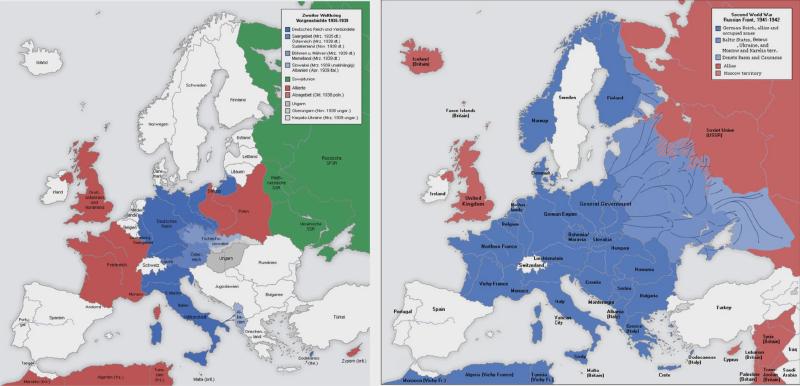
By the end of 1941, most of continental Europe had fallen to Nazi Germany and the other Axis powers, and by 1942, their forces had begun their significant advance in the eastern front deep into the Soviet Union. A key component of their rapid conquests was their revolutionary use of tanks in modern warfare. While other militaries, most notably that of France, used tanks as a modern armored form of cavalry, the Germans were the first to make full use of tanks’ speed and strength.

With the Nazis utilizing tanks with such devastating results, it was essential for the Allies to stop them. A key component of the solution was figuring out how many tanks the Germans had deployed in order to allocate resources effectively, since there was a tremendous danger both in underestimating and in overestimating the enemy’s strength. The consequence of underestimating is clear, since one could suddenly be outnumbered in battle. Overestimating is also bad, since it can lead to undue caution and failure to exploit advantages, or to committing too many resources in one theater and thus not having enough elsewhere. The Allies realized that the tanks destroyed and captured during a battle had serial numbers on their gearboxes that could help with this problem. With these data, the Allies found a statistical method to estimate the number of the tanks.

Methods

Now we gonna focus on searching for a good estimator for the number of the tanks. But before we start calculation, we should first clarify our criterion, that is, what properties are “good”? An intuitive idea is to find an unbiased estimator with as small variance as possible, and that is exactly what I’d pursue here. Then we may assume some key information for a deeper analysis. Suppose that Germany had $N$ tanks in total, and that the Allies observed $k$ tanks. Let the numbers of observed tanks be $x_{(1)},x_{(2)},\dots,x_{(k)}$ and $x_{(1)}<x_{(2)}<\dots<x_{(k)}$. Our goal is to find $\widehat{N}$, which is an estimator of $N$.

Method I

Now I’m going to demonstrate the original variant of the problem. Here we need another two assumptions that the first tank is numbered 1, and that the numbers are consecutive. What’s more, each tank has an equal chance of being observed. If we consider the numbers of observed tanks as a set of random variables $X_{(1)},X_{(2)},\dots,X_{(k)}$ ($X_{(1)}<X_{(2)}<\dots<X_{(k)}$), and $x_{(1)},x_{(2)},\dots,x_{(k)}$ as their observations, then we have $$ \Pr(X_{(k)}=x_{(k)})=\frac{x_{(k)}-1\choose k-1}{N \choose k}. $$ So $$ \mathbb{E}(X_{(k)})=\sum_{m=k}^{N}m\Pr(X_{(k)}=m)=\sum_{m=k}^{N}m\frac{m-1\choose k-1}{N \choose k} =k\sum_{m=k}^{N}\frac{m\choose k}{N \choose k}=\frac{k(N+1)}{k+1}, $$ $$ \mathbb{E}(X_{(k)}^2)=\sum_{m=k}^{N}m^2\frac{m-1\choose k-1}{N \choose k}= \sum_{m=k}^{N}(m+1)m\frac{m-1\choose k-1}{N \choose k}-\sum_{m=k}^{N}m\frac{m-1\choose k-1}{N \choose k} =\frac{k(N+1)(N+2)}{k+2}. $$ Here we use a trick, that is $\sum_{m=k}^N {m\choose k}={N+1\choose k+1}$. The fomula can be proven by induction. Rearranging the equality, we have $$ N=\left(1+\frac{1}{k}\right)\mathbb{E}(X_{(k)})-1. $$ So the point estimation of $N$ is $$ \widehat{N}=\left(1+\frac{1}{k}\right)X_{(k)}-1. $$ Let’s check some numerical characteristics of the estimator,

\[ \begin{aligned} \mathbb{E}(\widehat{N})&=\left(1+\frac{1}{k}\right)\mathbb{E}(X_{(k)})-1=N,\\ \mathrm{var}(\widehat{N})&=\left(1+\frac{1}{k}\right)^2\mathrm{var}(X_{(k)})\\ &=\left(1+\frac{1}{k}\right)^2\left(\mathbb{E}(X_{(k)}^2)-\left(\mathbb{E}(X_{(k)})\right)^2\right)\\ &=\frac{(N-k)(N+1)}{k(k+2)}. \end{aligned} \]

When $k\ll N$, the standard error of $\widehat{N}$ approximately equals to $N/k$. If the Allies observed more tanks, then the standard error will decrease rapidly. The fact is in accord with our intuition. Since we have only one observation of the random variable $X_{(k)}$, the result is satisfactory.

Method II

As we review the assupmtions of Method I, we may think of such a question - what if the first tank is not numbered 1? Method II is designed to remove this assumption. In this case, both the lowest serial number and the highest serial number are unknown to us, so we denote them as $N_1$ and $N_2$ respectively. Immediately we gain the identity $$ N=N_2-N_1+1. $$ Frome the identity we see that $N$ is determined by the difference between $N_2$ and $N_1$, so we can try to use the difference between $X_{(k)}$ and $X_{(1)}$. Now we define the spread $S=X_{(k)}-X_{(1)}$ and hence the observerd spread $s=x_{(k)}-x_{(1)}$. Then we have $$ \Pr(S=s)=\frac{\sum_{x_{(1)}=N_1}^{N_2-s}{s-1\choose k-2}}{N\choose k}=\frac{(N_2-s-N_1+1){s-1\choose k-2}}{N\choose k}=\frac{(N-s){s-1\choose k-2}}{N\choose k}. $$ As what we’ve done in Method 1, we are interested in $\mathbb{E}(S)$ and $\mathrm{var}(S)$. Before we start to calcute these two numerical characteristics, let’s first figure out some equations to make our calculation easier:

\[ \begin{aligned} \Sigma_1&=\sum_{s=k-1}^{N-1}s{s-1\choose k-2}=(k-1)\sum_{s=k-1}^{N-1}s{s\choose k-1}=(k-1){N\choose k},\\ \Sigma_2&=\sum_{s=k-1}^{N-1}(s+1)s{s-1\choose k-2}=k(k-1)\sum_{s=k-1}^{N-1}s{s+1\choose k+1}=k(k-1){N+1\choose k+1},\\ \Sigma_3&=\sum_{s=k-1}^{N-1}(s+2)(s+1)s{s-1\choose k-2}=(k+1)k(k-1)\sum_{s=k-1}^{N-1}s{s+2\choose k+2}\\&=(k+1)k(k-1){N+2\choose k+2}. \end{aligned} \]

Then, it is easy to find that

\[ \begin{aligned} \mathbb{E}(S)&=\sum_{s=k-1}^{N-1}s\Pr(S=s)=\sum_{s=k-1}^{N-1}\frac{s(N-s){s-1\choose k-2}}{N\choose k}=\frac{(N+1)\Sigma_1-\Sigma_2}{N\choose k}\\&=\frac{(N+1)(k-1)}{k+1},\\ \mathbb{E}(S^2)&=\sum_{s=k-1}^{N-1}s^2\Pr(S=s)=\sum_{s=k-1}^{N-1}\frac{s^2(N-s){s-1\choose k-2}}{N\choose k}=\frac{(N+3)\Sigma_2-(N+1)\Sigma_1-\Sigma_3}{N\choose k}\\&=\frac{(kN+k-2)(N+1)(k-1)}{(k+1)(k+2)}. \end{aligned} \]

So the point estimation of $N$ is $$ \widehat{N}=\frac{k+1}{k-1}S-1, $$ and we have

\[ \begin{aligned} \mathbb{E}(\widehat{N})&=\frac{k+1}{k-1}\mathbb{E}(S)-1=N,\\ \mathrm{var}(\widehat{N})&=\left(\frac{k+1}{k-1}\right)^2\mathrm{var}(S)\\ &=\left(\frac{k+1}{k-1}\right)^2\left(\mathbb{E}(S^2)-\left(\mathbb{E}(S)\right)^2\right)\\ &=\frac{2(N-k)(N+1)}{(k-1)(k+2)}. \end{aligned} \]

Compared to Method I, the variance of the estimator in Method II is about twice as much as that of the estimator in Method I. It seems that Method I is better. However, remind that in Method I, we have one more assumption. If the assumption is true, then the estimator I is better since the estimator II neglects the useful information, which makes it possess bigger variance. But if the assumption is not true, then the estimator I is not necessarily an unbiased estimation since all the deduction is based on the wrong assumption! Thus, we can hardly tell which etimator is better and the choice depends on your criterion.